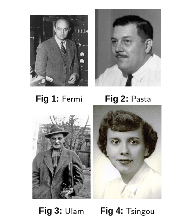
Continuing the lazy turn of events, the second blog on my very “frequently updated” website, is brought to you by another term project of mine, courtesy of my Non linear Dynamics professor and the geniuses over at Los Alamos,namely Enrico Fermi, John Pasta, Stanislaw Ulam and Mary Tsingou. More commonly known as the FPUT problem, the methods used and the conclusions reached in this paradox-of-the-decade have heralded the age of computational physics and a more nuanced study of CHAOS.

I had submitted a report for evaluation of the term project, which I have, similar to my previous blog, converted from LaTex to Markdown using the All-Mighty pandoc. So I invite you to brew a cup of masala chai, put your glasses on, and start reading this terribly written blogpost of mine.

History

In light of the new MANIAC(Metropolis and von Neumann Install Awful Computers, acronym courtesy Gamow) computer, Fermi, Pasta, Ulam, and Tsingou[13] set out to study some physical problem using numerical simulations. They chose to study a 1D chain of particles connected by nonlinear springs. Their goal was to understand how energy would distribute among the normal modes of the system over time, expecting that the nonlinearity would lead to thermalization and equipartition of energy among the modes.

We first introduce the FPUT problem and its original expectations. Then we will gloss over the backdrop of hamiltonian systems and ergodicity. Finally, we will discuss the surprising results. Then we try to answer some questions that arise from the problem. Then we try to see some possible solutions to the problem. Finally, we connect the richness of this problem with statistical mechanics. For this, we will use [5] and [1] as our main references.

For the more interested reader with higher levels of motivation and reading prowess than the nincompoop author of this blog, can also refer to the extensive review by Giovanni Gallavotti[6]

Problem Setup

The FPUT problem considers a one-dimensional chain of \(N\) particles connected by springs with linear and nonlinear restoring forces. The Hamiltonian is as follows:

\[H = \sum_{i=1}^{N} \frac{p_i^2}{2} + \sum_{i=1}^{N} \left( \frac{1}{2} (x_{i+1} - x_i)^2 + \frac{\alpha}{3} (x_{i+1} - x_i)^3 + \frac{\beta}{4} (x_{i+1} - x_i)^4 \right)\]

where \(p_i\) is the momentum of the \(i^{th}\) particle, \(x_i\) is its position, and \(\alpha, \beta\) are the coefficients for the nonlinear terms. The boundary conditions are fixed at both ends: \(x_0 = x_{N+1} = 0\). The equations of motion derived from the Hamiltonian are given by:

\[\begin{align*} \frac{d^2 x_i}{dt^2} = (x_{i+1} - 2x_i + x_{i-1}) + \alpha \left( (x_{i+1} - x_i)^2 - (x_i - x_{i-1})^2 \right) + \beta \left( (x_{i+1} - x_i)^3 - (x_i - x_{i-1})^3 \right) \end{align*}\]

for \(i = 1, 2, \ldots, N\), with appropriate boundary conditions.

Normal Modes

For the linear Hamiltonian \((H_0)\) , we can express the displacements in terms of the normal mode coordinates \(Q_k\):

\[Q_k(t) = \sqrt{\frac{2}{N+1}} \sum_{j=1}^{N} x_j(t) \sin\left(\frac{\pi k j}{N+1}\right)\]

where \(k = 1, 2, \ldots, N\). Each normal mode oscillates with its own frequency \(\omega_k\):

\[\omega_k = 2 \sin\left(\frac{\pi k}{2(N+1)}\right)\]

The normal mode coordinates are easily found using the Fourier expansion and plugging in the appropriate boundary conditions. Using the normal mode coordinates, the equations of motion for the linear system can be written as:

\[\ddot{Q}_k + \omega_k^2 Q_k = 0\]

with the \(k^{th}\) mode energy given by:

\[E_k = \frac{1}{2} \dot{Q}_k^2 + \frac{1}{2} \omega_k^2 Q_k^2\]

Thus, we can decouple the oscillators in the linear case. No energy exchange between modes. The original Hamiltonian with linear springs \((H_0)\) would lead to normal modes of vibration, each with a specific frequency. The expectation was that the addition of nonlinear terms\((H_1)\) with perturbation, either \(\alpha\) or \(\beta\), would cause the energy to spread out among these modes over time, leading to thermalization and equipartition of energy.

For the \(\alpha\) model, the equations of motion in terms of normal modes become:

\[\ddot{Q}_k + \omega_k^2 Q_k = -\frac{\alpha}{\sqrt{2(N+1)}} \sum_{j,l=1}^{N} C_{j l k} Q_j Q_l Q_m\]

where \(C_{j l k}\) are coupling coefficients that depend on the mode indices. Similarly, for the \(\beta\) model, we have:

\[\ddot{Q}_k + \omega_k^2 Q_k = -\frac{\beta}{2(N+1)} \sum_{j,l,m=1}^{N} D_{j l m k} Q_j Q_l Q_m Q_n\]

where \(D_{j l m k}\) are the corresponding coupling coefficients.

A Classical Mechanics Refresher

A constant of motion is a function \(F(q_i, p_i, t)\) that remains constant along the trajectories of the system in phase space for a given Hamiltonian \(H(q_i, p_i, t)\). Mathematically, \(F\) is a constant of motion if its total time derivative vanishes:

\[\frac{dF}{dt} = \frac{\partial F}{\partial t} + \{F, H\} = 0\]

For example, in a system with a time-independent Lagrangian, the Hamiltonian itself is a constant of motion, representing the total energy of the system.

Integrability

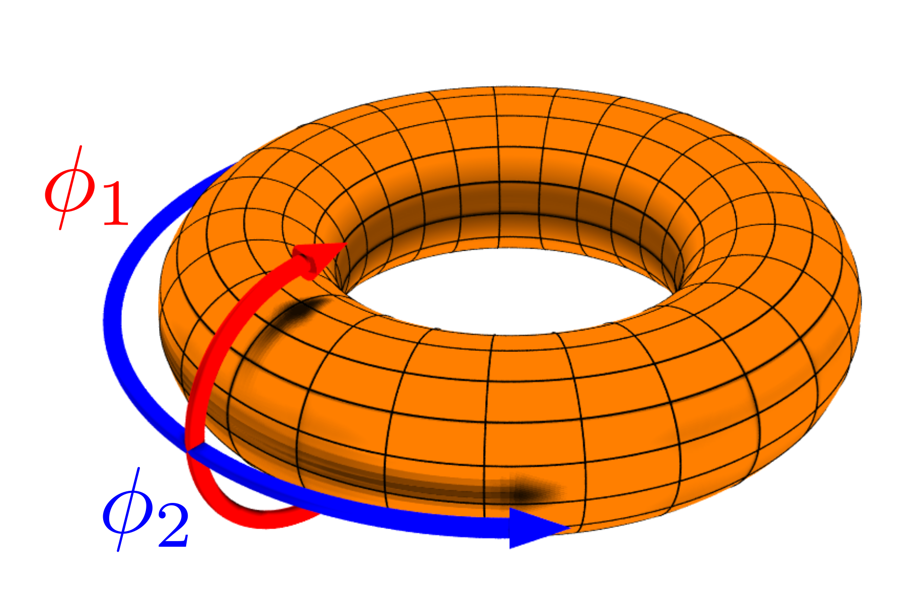
A Hamiltonian system with \(N\) degrees of freedom is said to be integrable if it possesses \(N\) independent constants of motion. In such systems, the equations of motion simplify significantly, and the dynamics can be described as linear motion on an invariant tori in phase space.

More formally, a Hamiltonian \(H(q_i, p_i)\) is integrable if there exists a single-valued analytical canonical transformation to action-angle variables \((J_i, \theta_i)\) such that the Hamiltonian depends only on the action variables:

\[H = H(J_1, J_2, \ldots, J_N)\]

In these variables, the equations of motion become:

\[J_i = J_{i0}, \quad \theta_i = \omega_i(J) t + \theta_{i0}\]

where \(\omega_i(J) = \frac{\partial H}{J_i}\) are the frequencies of the system. This motion can be mapped to an invariant torus in the appropriate phase space. The action represents radii of the tori, while the angle variable describes the evolution on the surface of the tori.

A result a la Poincaré

Consider perturbed Hamiltonians of the form:

\[H(J, \theta) = H_0(J) + \epsilon H_1(J, \theta)\]

where \(\epsilon\) is a small parameter, \(H_0(J)\) is integrable, and the frequencies of the unperturbed hamiltonian \(\omega_i = \frac{\partial H_0}{J_i}\) are functionally independent.

A nice sketch of this proof can be seen at [5]. Basically, when Poincaré starts with the Hamiltonian \(H = H_0 + \mu H_1\). Then he looks for constants of the motion of the form:

\[\Phi(Q, P,\mu) = \sum_{k=0}^\infty \Phi(Q,P)\]

where \(Q,P\) are the position and momentum variables and where all \(\Phi_k\) are all analytic functions of \(Q,P\). Specifically, since \(\Phi\) is a constant of the motion, he inserts the above expression in the Poisson Bracket equation \(\{H,\Phi\} = 0\) and then insists that for each coefficient of each \(\mu^k\) equal to zero. This yields \(\{H_0,\Phi_0\} = 0\), which means \(\{H_0,\Phi_k\} = - \{H_0, \Phi_{k-1}\} ~ \forall ~ k>0\). We can solve these equations iteratively for all \(\Phi_k\) once \(\Phi_0\), which is a constant of motion for the integrble Hamiltonian, is specified. Poincaré wants to analytically continue \(\Phi_0\). Then he shows that this is not possible due to the presence of denominators which become zero for a dense set of hypersurfaces. As a result, the only constant of motion that can be analytically continued is the Hamiltonian itself.

Fermi’s Proof

Fermi started out his career trying to prove the ergodic hypothesis. He proved that the class of Poincaré-type Hamiltonians are ergodic. The proof sketch is quite straightforward. He proceeds via contradiction. Suppose, the system is not ergodic. In consequence, at least two distinct regions of phase space exist that are invariant under Hamiltonian flow. Fermi now asserts that there must a surface separating these two regions. This surface must be a constant of motion, since the Hamiltonian flow cannot cross it. However, by Poincaré’s result, no such constant of motion exists for Poincaré-type Hamiltonians. Therefore, the system must be ergodic. The problem with this proof is that Fermi assumed that the separating surface is analytic, which is not necessarily true. The KAM theorem shows that these surfaces are disjoint sets that fill most of the phase space, but are not analytic.

Under a canonical transformation, the FPUT Hamiltonian can be expressed as a Poincaré-type Hamiltonian. Therefore, by Fermi’s proof, the FPUT system is ergodic. We cannot measure ergodicity directly. However, since Fermi’s Proof dictates that the FPUT system is ergodic, and therefore should follow the principle of equal a priori probabilities. This would imply that over long times, the law of equipartition of energy should hold. This is how the original authors wanted to verify Fermi’s proof.

A more detailed explanation of this connection will be provided later in the report.

The Problem with The Problem

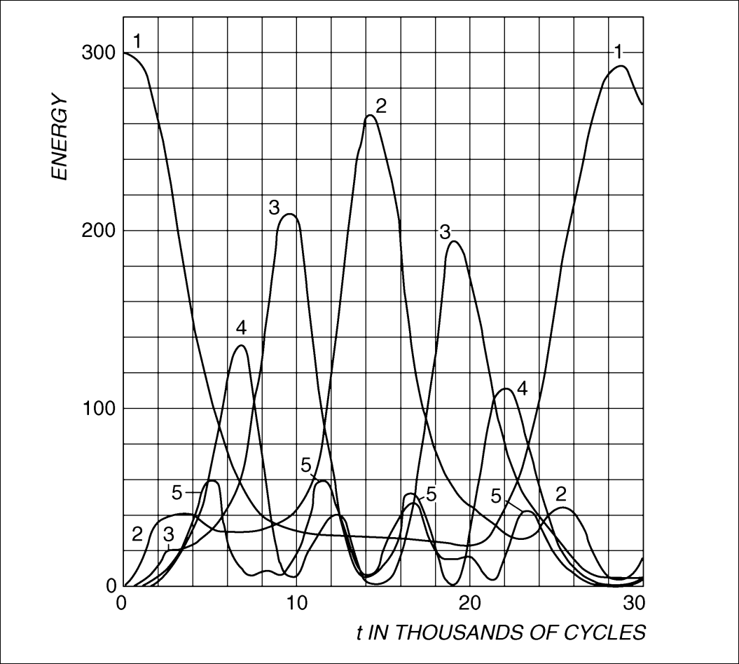
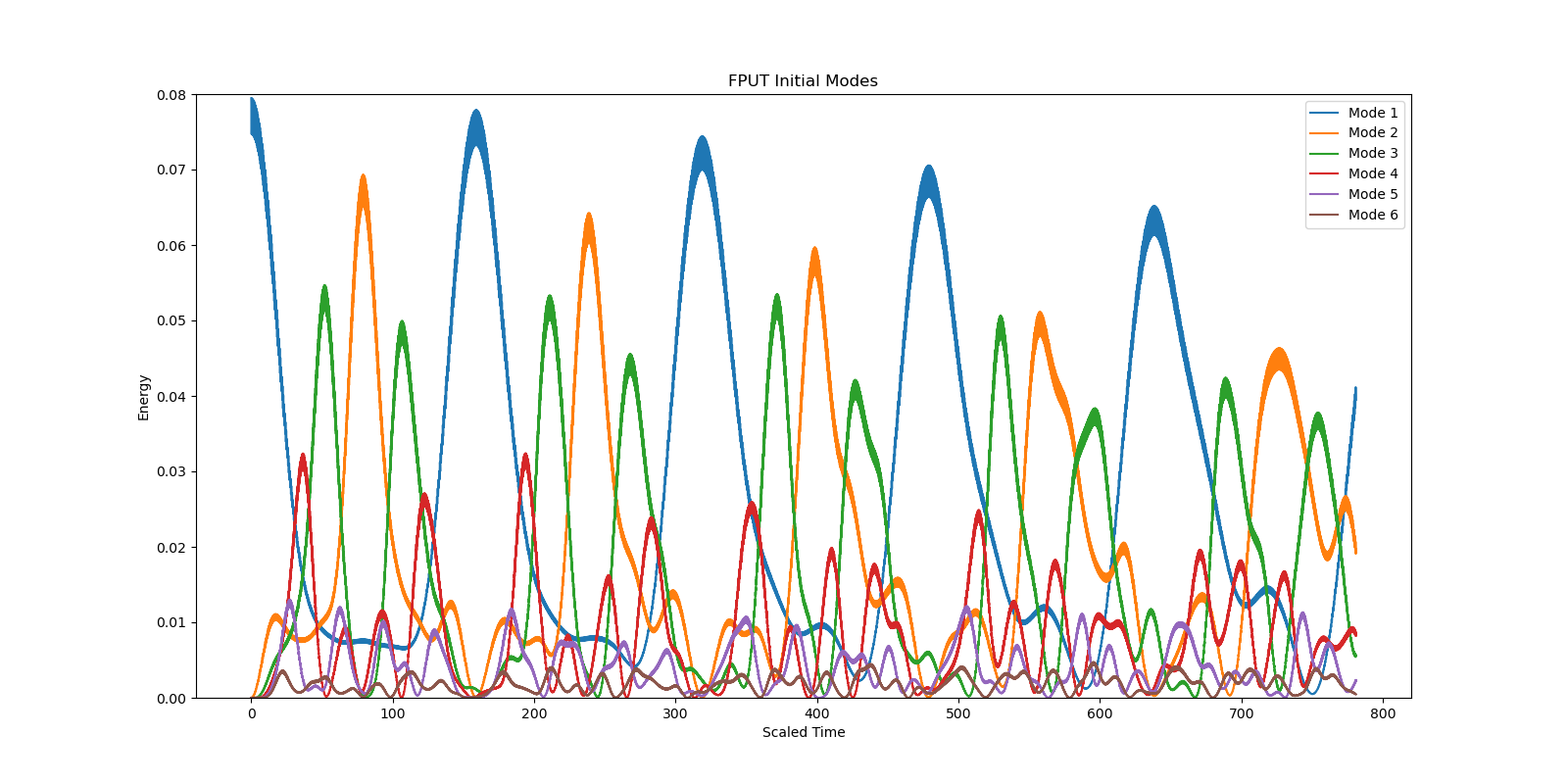
However, the numerical simulations by Fermi, Pasta, Ulam and Tsingou showed that the system did not thermalize as expected. Instead of energy spreading out evenly among all modes, it exhibited a phenomenon known as "recurrence," where the energy returned to the initially excited mode after some time.

Numerical Simulation

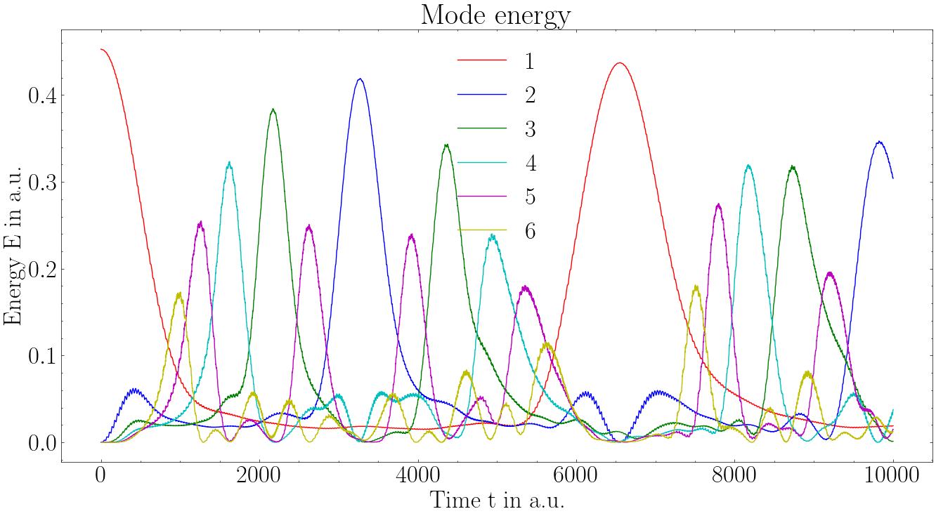
To verify the results of Fermi, Pasta, Ulam and Tsingou, we perform our own numerical simulations of the FPUT system. We used both Euler and Velocity-Verlet integration methods to solve the equations of motion.

• The Euler method is a simple first-order method, but it can be less accurate and does not conserve energy well over long simulations.

• The Velocity-Verlet method is a second-order symplectic integrator that is more accurate and better at conserving energy in Hamiltonian systems.

  A nice handout on these simulations can be found at [7]

Euler Method

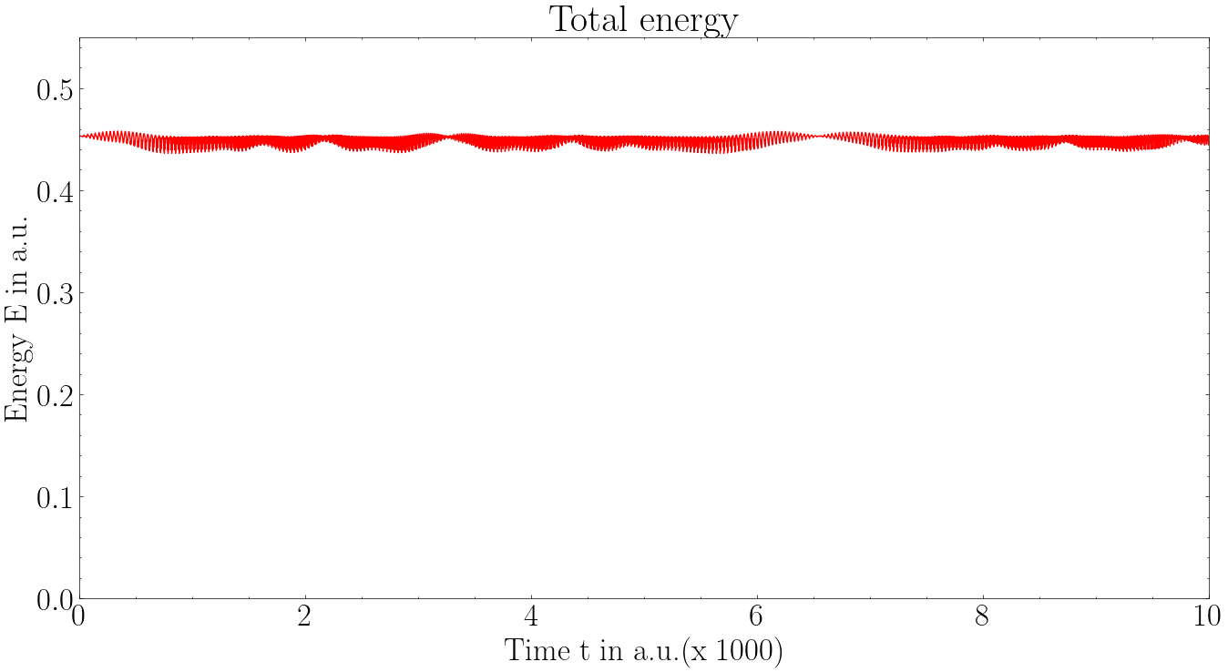
Velocity Verlet

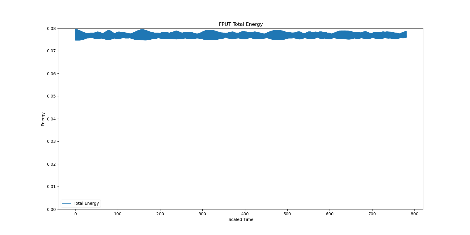
We have seen that the numerical simulations do not match the theoretical predictions by the original creators of this model. There are some questions that need to answered, in light of this discrepancy between the theoretical and numerical predictions.

Fermi’s Folly

The proof by Fermi has been shown to be incorrect. To see this, a landmark theorem by Kolmogorov, Arnold and Moser is required.

The KAM theorem provides a resolution to why the FPUT system does not thermalize for small perturbations. The surviving invariant tori still show signatures of integrable behavior, preventing ergodicity. Fermi in his proof assumed that the surface dividing the regions of phase space invariant under Hamiltonian flow, is analytic. The work by Kolmogorov, shows that these surfaces are not analytic, and are in fact "pathological monstrosities".

Inquisitions

We try to answer some questions that can be asked and people have studied.

• Is the FPUT system integrable or non-integrable? Note Poincaré’s result states that we can’t analytically continue the constants of motion from the unperturbed system to the perturbed system. It does not say anything about introducing new constants of motion.

• Does the FPUT system not thermalize at all, or does it thermalize over very long timescales?

• Does the FPUT system thermalize for certain initial conditions and not for others?

• Is the FPUT system ergodic after all?

Let’s explore these questions one by one.

Is the FPUT system integrable or non-integrable?

People have thought for some time that the FPUT system might be integrable after all. However, the simple answer to our question is NO. Let us consider the \(\alpha\) model with \(N=3\) masses with periodic boundary conditions. The Hamiltonian is given by:

\[H = \sum_{i=1}^{3} \frac{p_i^2}{2} + \sum_{i=1}^{2} \left( \frac{1}{2} (x_{i+1} - x_i)^2 + \frac{\alpha}{3} (x_{i+1} - x_i)^3 \right)\]

Under a simple canonical transformation, we obtain the Hénon-Heiles Hamiltonian, which is a well known non-integrable system, that exhibits chaotic behavior above a certain energy threshold.

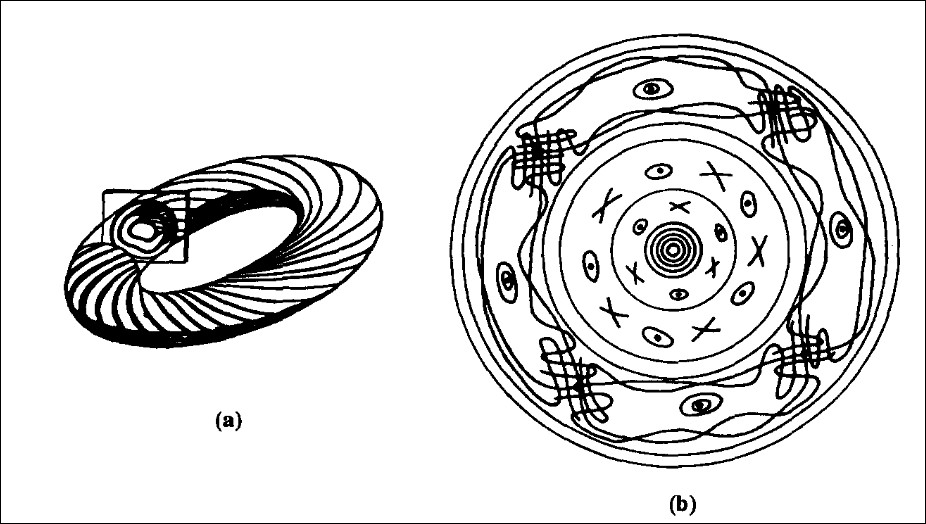
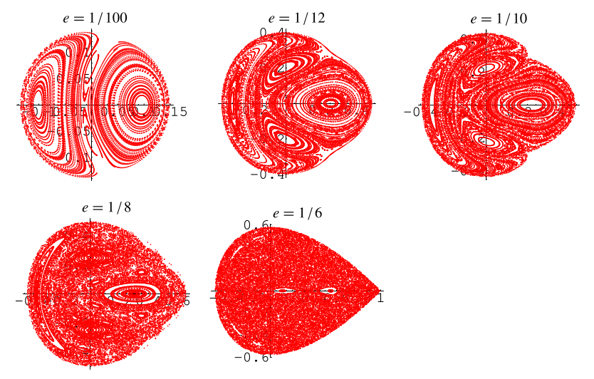
Hénon Heiles Hamiltonian

The Hénon-Heiles Hamiltonian is given by:

\[H = \frac{1}{2} (p_x^2 + p_y^2) + \frac{1}{2} (x^2 + y^2) + x^2 y - \frac{1}{3} y^3\]

This system was originally proposed to model the motion of a star around a galactic center. For energies above a certain threshold, the system exhibits chaotic behavior, with trajectories that are highly sensitive to initial conditions.

As a result, we get a clue that the FPUT system might be chaotic for higher perturbations or energies.

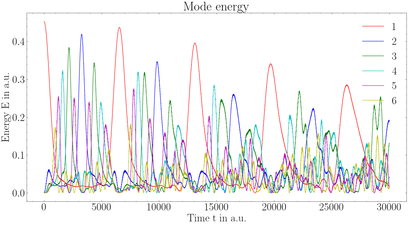
Does the FPUT system not thermalize at all, or does it thermalize over very long timescales?

After some time of evolution, we see a dip in the energy of the first mode. People had conjectured that over longer timescales, the system might thermalize.

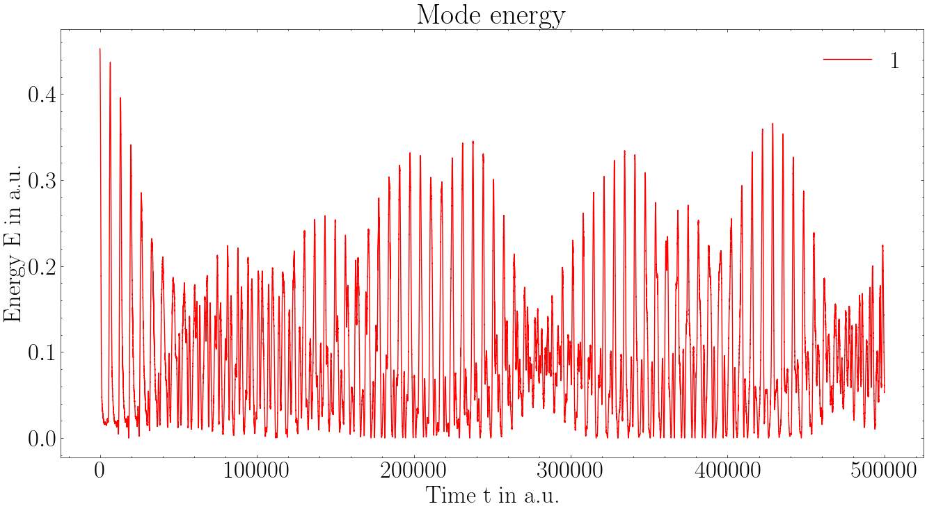
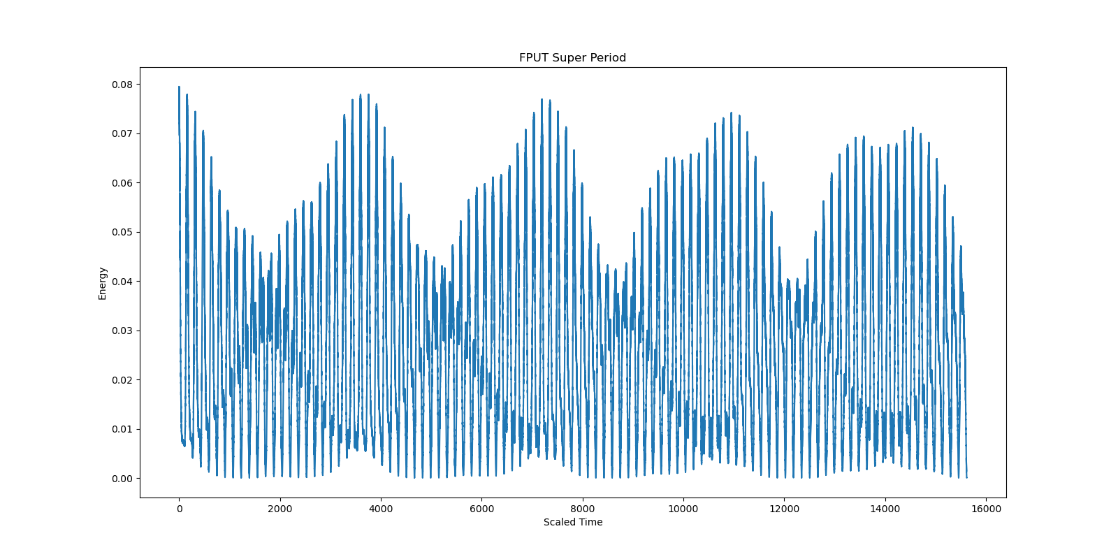
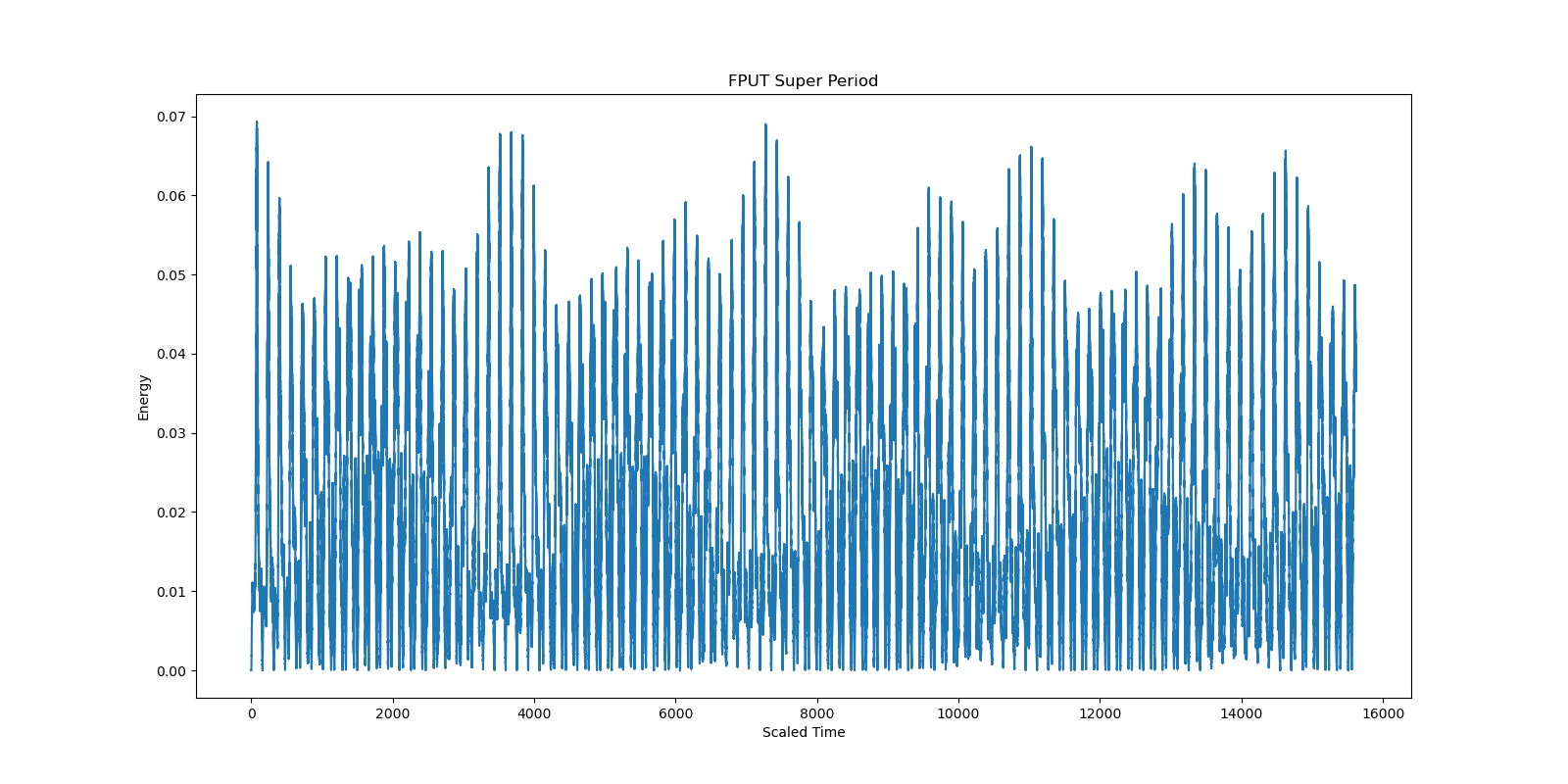
Super Period

Even though there an energy dip after some time, after observing a bit longer, we see some sort of super recurrence. Almost all of the energy( over 99%) flows back into the first mode. The super period was first observed by Tuck and Tsingou(then Menzel) in 1972.

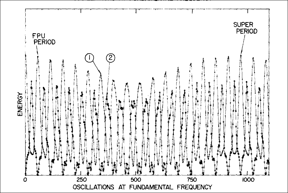
We simulated the same using both Euler and Velocity Verlet algorithms. We observe super periods in both methods, however for the euler method, quite less than 99% of energy returns to the first mode. This problem has been eliminated when the velocity verlet method is used.

There have been some studies that suggest that the FPUT system might thermalize over extremely long timescales. Similar to glassy behavior in condensed matter systems, the FPUT system might be stuck in a metastable state for long times before eventually reaching thermal equilibrium. KAM theorem hints that for small perturbations, there are invariant tori that survive. Therefore, for initial conditions lying on these tori, the system will not thermalize. Building on this Idea F.M. Izrailev and B.V. Chirikov proposed the stochasticity threshold, also called the Chirikov criterion[4]. According to this criterion, when the perturbation strength exceeds a certain threshold, the invariant tori break down, leading to widespread chaos in phase space and subsequent thermalization.The original FPUT paper considers two models, the \(\alpha\) and \(\beta\) models, with certain initial conditions. Israilev and Chirikov showed for the \(\beta\) model,the initial conditions lie below the stochasticity threshold for the respective models, explaining the lack of thermalization.

There is region of conditions where due to the KAM theorem, the system does not thermalize. This criterion is a property of a lot of other systems as well. The system here exhibits Kolmogorov Stability. The criterion shows that very high nonlinear couplings are required for thermalization when low frequency modes are excited initially. For higher modes and large \(N\), the threshold is much lower, and thermalization can occur for smaller nonlinear couplings.

Resolutions

Which neighbour is Integrable?

This energy recurrence phenomenon is explained by the fact that there is an integrable Hamiltonian in the neighbourhood of the FPUT system.(We can map a Hamiltonian to a space where this sentence makes perfect sense). That cannot be the linear model, since the Poincare surfaces of the FPU are quite different from that of the linear one. In the quest for finding a suitable candidate, two of them have been the leading candidates,

1. The KdV equation.

2. The toda Lattice

The KdV Equation

We shall look at the connection to the KdV equation in more detail. The FPUT system can be regarded a discrete approximation to the integrable Korteweg-de Vries (KdV) equation. Let’s see how. We shall consider the \(\alpha\) model for simplicity. The connection to the KdV equation is a tiny bit technical, so bear with me. We will show that the naive approach to the continuum limit does not work, and leads to unphysical results. We follow the approach by [12].

The FPUT equations of motion for the \(\alpha\) model with arbitrary \(m\) and \(k\) are given by:

\[m \ddot{x}_i = k (x_{i+1} - 2x_i + x_{i-1})\left(1 + \alpha (x_{i+1} - x_{i-1}) \right)\]

We approximate the spring mass system as a continuous string of length L. Let the equilibrium positions of the masses be given by \(x_i^0 = ih\), where \(h = L/(N+1)\) is the spacing between masses. Denote \(\rho\) is the density of the string, then \(m = \rho h\). Let \(\kappa\) denotes the Young’s modulus for the string (i.e., the spring constant for a piece of unit length) Then k = \(\kappa/h\) will be the spring constant for a piece of length h.

Defining \(c = \sqrt{\kappa/\rho}\) we obtain,

\[\ddot{x}_i = c^2 \frac{(x_{i+1} - 2x_i + x_{i-1})}{h^2}\left(1 + \alpha (x_{i+1} - x_{i-1}) \right)\]

Let \(u(x,t)\) be the function measuring the displacement of the string from equilibrium at position \(x\) and time \(t\). Let us analyse for one particular \(x=x_i\) Then,

• \(x_i(t) = u(x, t)\)

• \(x_{i+1}(t) = u(x + h, t)\)

• \(x_{i-1}(t) = u(x - h, t)\)

We can see that \(\ddot{x}_i = u_{tt} (x, t)\). Using Taylor series expansion about \(x\), we have,

\[\frac{(x_{i+1} - 2x_i + x_{i-1})}{h^2} = u_{xx}(x, t) + u_{xxxx}(x, t) \frac{h^2}{12} + O(h^4)\]

Similarly,

\[\alpha (x_{i+1} - x_{i-1}) = (2 \alpha h )u_x(x, t) + \frac{2 \alpha h^3}{6} u_{xxx}(x, t) + O(h^5)\]

We arrive at,

\[\left(\frac{1}{c^2}\right) u_{tt} - u_{xx} = \epsilon u_x u_{xx} + O(h^2)\]

where \(\epsilon = 2 \alpha h\). We obtain the PDE,

\[u_{tt} = c^2(1 + \epsilon u_x )u_{xx}\]

One can draw parallels between this equation and the inviscid Burgers equation, which is known to develop shocks in finite time, for generic initial conditions. For wave like solutions, the rising part of the wave with goes faster with \(u_x > 0\) than the fallling part with \(u_x < 0\), leading to wave steepening and shock formation. One can see how following the inviscid Burgers equation develops shocks over a finite time. This happens over a characteristic time scale \(t_s\) which is found to be much smaller than the recurrence time observed in the FPUT simulations.

This is unphysical, since the FPUT system with small nonlinearity does not exhibit such shock formation. To resolve this issue, we follow the approach by Zabusky and Kruskal. The correct approach is to keep higher order terms in the Taylor series expansion. Keeping terms upto order \(h^2\), we obtain the PDE,

\[\frac{1}{c^2} u_{tt} = (1 + 2 \alpha h u_x )u_{xx} + \frac{ h^2}{12} u_{xxxx} + O(h^4) \tag{KZ}\]

The additional fourth order derivative term acts as a dispersive term, preventing shock formation. We now differentiate w.r.t. \(x\) and define \(w = u_x\), to obtain,

\[\frac{1}{c^2} w_{tt} = w_{xx} + \alpha h \frac{\partial^2}{\partial w \partial x} + \frac{h^2}{12} w_{xxxx} + O(h^4)\]

This is known as the Boussinesq equation. This admits wave like solutions that do not form shocks, these are periodic water waves.

Note that for small values \(\alpha\) and \(h\), the wave like solutions should qualitatively behave like solutions to the linear wave equation. In general, the solutions will be superpositions of right and left moving waves. Here, these two cases are treated differently. To be specific, let us consider only right moving waves. We would like to look for solutions, such that behave more and more like right moving waves for longer and longer times as \(\alpha, h \to 0\).

To interpret this physically, the function \(u(x,t) = y(x - ct, \alpha h c t)\) uniformly approximates the right moving wave \(u^0(x,t) = y(x - ct, \alpha h c t_0)\) over the time interval \(|t - t_0| < T\). To restate this, \(u(x,t) = y(x - ct, \alpha h c t)\) is approximately a right moving wave whose shape gradually changes over time.

We now substitute \(w(x,t) = y(x - ct, \alpha h c t)\) into the (KZ) equation, and divide by \(- 2 \alpha h\). Neglecting terms of order \(O(h^4)\), we obtain the equation,

\[y_{\xi \tau} - \left(\frac{\alpha h}{2}\right) y_{\tau \tau} = -\frac{h^2}{24} y_{\xi \xi \xi \xi} - y_\xi y_{\xi \xi}\]

We begin by making the substitutions, \(\xi = x - ct\) and \(\tau = \alpha h c t\). Now, we can pass it into the continuum limit \(\alpha, h \to 0\). We assume that \(h\) and \(\alpha\) are related such that \(\alpha, h \to 0\) and \(h/\alpha\) tend to a positive limit. We then define \(\delta = \lim_{h \rightarrow 0} \sqrt{\frac{h}{24 \alpha}}\). This also means that \(\alpha h = O(h^2)\).

\[\begin{align*} \frac{\partial^k}{\partial x^k} = \frac{\partial^k}{\partial \xi^k} ~~;~~ \frac{\partial}{\partial t} = -c \frac{\partial \xi} + \alpha h c \frac{\partial}{\partial \tau} \\ \frac{\partial^2}{\partial t^2} = c^2 \frac{\partial^2}{\partial \xi^2} - 2 \alpha h c^2 \frac{\partial^2}{\partial \xi^2}{\tau}+ (\alpha h c)^2 \frac{\partial^2}{\partial \tau^2} \end{align*}\]

Our wave operator reduces to

\[\frac{1}{c^2} \frac{\partial^2}{\partial t^2} - \frac{\partial^2}{\partial x^2} = - 2 \alpha h \frac{\partial^2}{\partial \xi \partial \tau} + (\alpha h)^2 \frac{\partial^2}{\partial \tau^2}\]

In this limit, we obtain the celebrated Korteweg-de Vries Equation by taking \(v(\xi, \tau) = y_\xi(\xi, \tau)\):

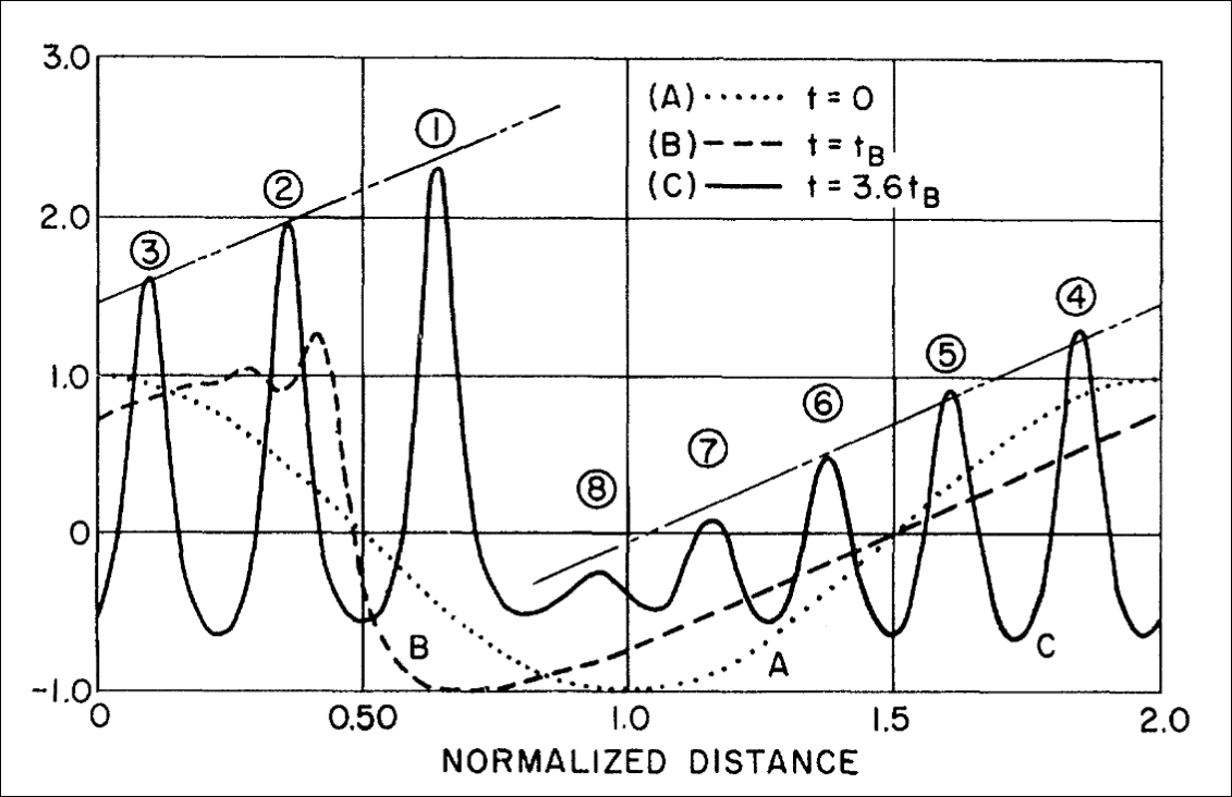
\[v_\tau + v v_\xi + \delta^2 v_{\xi \xi \xi} = 0\]

In their seminal 1965 paper, Zabusky and Kruskal performed numerical simulations of the KdV equation and discovered solitons, which are stable, localized wave packets that maintain their shape while traveling at constant speed. They then observed how solitons interfere with each other, and found that they pass through each other without changing shape. Using this connection to solitons, they gave a phenomenological explanation for the recurrence phenomenon observed in the FPUT system. We now see how these solitons arise in the KdV equation, from a small section of the report [8].

Initially, the first two terms of the KdV equation dominate and the classical overtaking phenomenon occurs; that is, \(u\) steepens in regions where it has a negative slope. Second, after \(u\) has steepened sufficiently, the third term becomes important and serves to prevent the formation of a discontinuity. Instead, oscillations of small wavelength (of order \(\delta\)) develop on the left of the front. The amplitudes of the oscillations grow and finally each oscillation achieves an almost steady amplitude (which increases linearly from left to right) and has a shape almost identical to that of an individual solitary-wave solution of the KdV equation. Finally, each such "solitary-wave pulse"or "soliton" begins to move uniformly at a rate (relative to the background value of u from which the pulse rises) which is linearly proportional to its amplitude. Thus, the solitons spread apart. Because of the periodicity, two or more solitons eventually overlap spatially and interact nonlinearly. Shortly after the interaction, they reappear virtually unaffected in size or shape. In other words, solitons "pass through" one another without losing their identity.

Here we have a nonlinear physical process in which interacting localized pulses do not scatter irreversibly.

They explained the recurrence phenomenon on an FPUT system with periodic boundary conditions. These solitons arise and interfere periodically, leading to the recurrence of the initial state after some time. Note that these derivation also agrees with the Chirikov criterion. The KdV approximation is valid for small nonlinearity, which is precisely the regime where the stochasticity threshold is high, preventing thermalization.

Toda Lattice

The N-particle Toda lattice also serves as a leading candidate as an integrable Hamiltonian in the neighbourhood of the FPUT lattice.

\[H = \frac{1}{2} \sum P_k^2 +\frac{1}{2} \left(\sum \exp\left(Q_{k} - Q_{k-1}\right) \right)\]

where the index \(k\) runs from \(1\) to \(N\) and we impose periodic boundary consitions \(Q_{N+1} = Q_1\). The Toda lattice can be in a sense, the discretized form of the KdV equation. One can show that the Toda Lattice is completely integrable using LAX pairs.

Connection to Statistical Mechanics

Statistical mechanics has been one the most successful theories in physics. It provides a microscopic explanation for macroscopic thermodynamic phenomena, for widly different systems. Even after more than a century after Boltzmann’s pioneering work, the foundations of statistical mechanics are still not quite rigourously justified. Some of them include what the thermodynamic limit really means, whether the free energy functionals are well defined at that limit, why do these systems thermalize, and most importantly, the ergodic hypothesis. One might think it would be too naive to apriori expect equipartition of energy in a slightly perturbed system. But if we establish a connection between ergodicity and the basic building block of statistical mechanics, the principle of equal a priori probabilities, we can see why the FPUT problem is so rich in its physical implications.

Ergodicity

This is a restatement of the hypothesis that Boltzmann used to derive the microcanonical ensemble and the law of equipartition of energy. Let’s see a heuristic proof of this statement.

Consider a system with Hamiltonian \(H(q_i, p_i)\) and total energy \(E\). Let us discretize the phase space into small cells of volume \(\Delta V_\Gamma\). The total time spent by the system in a cell \(\Delta V_\Gamma\) over a long time \(T\) is given by:

\[\tau \propto \Delta V_\Gamma\]

Therefore, the probability of finding the system in that cell, in our long time observation is given by:

\[P(\Delta V_\Gamma) = \frac{\tau}{T} \propto \Delta V_\Gamma\]

Taking the limit \(\Delta V_\Gamma \to 0\), we obtain the probability density function:

\[dP = \rho(q_i, p_i) dV_\Gamma \propto dV_\Gamma\]

This principle is the cornerstone of statistical mechanics. It allows us to derive the microcanonical ensemble and subsequently other ensembles. The previous definition has a certain nuance that is often overlooked. The word accessible is very important here. The microcanonical ensemble is,generally, defined for an isolated system with fixed total energy \(E\). Suppose for a system which has an additional constant of motion \(\Phi(p_i, q_i)\) . Then for a certain initial condition, both \(H(p_i, q_i)\) and \(\Phi(p_i, q_i)\) will be conserved. Therefore, our energy hypersurface will be further constrained to a submanifold defined by \(\Phi(p_i, q_i) = \phi_0\). So the probability density function will be given by:

\[dP \propto \delta(H(p_i, q_i) - E) \delta(\Phi(p_i, q_i) - \phi_0) dV_\Gamma\]

We need to ensure that there are no additional constants of motion other than the Hamiltonian itself, to obtain the microcanonical ensemble in its widely used form. Recall that Poincaré’s result states that for perturbed Hamiltonians of that form, there exists no constant of motion \(\Phi(Q_k, P_k, t)\) that is analytic in \(Q_k, P_k\) and \(\epsilon\), other than the Hamiltonian itself. This motivated Fermi’s proof to show that those Hamiltonians are ergodic. The Ergodic hypothesis also helps us understand systems and their validity in the real world. This relates time averages to ensemble averages.

\[\overline{A} = \lim_{T \to \infty} \frac{1}{T} \int_0^T A(q(t), p(t)) dt = \langle A \rangle = \int A(q, p) \rho(q, p) dV_\Gamma\]

For real systems, we can only measure time averages. The ergodic hypothesis allows us to equate these to ensemble averages, which are easier to compute theoretically. A proof of this hypothesis still eludes us. There have been some system specific proofs, by von Neumann and Birkhoff, but a general proof is still unknown.

Energy Equipartition

The principle of equal a priori probabilities leads to the law of equipartition of energy. This is a fairly standard derivation. One can look at any statistical mechanics textbook for details, for example [9]. Since equipartition of energy is a direct consequence of the principle of equal a priori probabilities, FPUT decided to test this as a signature of ergodicity in their system.

Remarks

The foundations of statistical mechanics are still not completely rigourously justified. Khinchin [10] and Ruelle [11] have a lot of opinions and criticisms about these foundations. The FPUT problem is a classic example that highlights the subtleties involved in these justifications. It launched the fields of studying solitons and chaos theory.

Moreover, FPUT forever pioneered the usage of computers in physics research.

That’s all folks

Initially the experiment was widely referred to as the FPU problem, since Mary Tsingou was only recognised in a footnote for all the programming done for this experiment. A very illuminating read about the problem focusing on giving the deserving credits to Mrs. Mary Tsingou Menzel is here. Unlike my previous blogpost, I shall end with a relevant quote.

                       We thank Miss Mary Tsingou

Danke Schön

Feel free to direct your feedback and curses to my email: iamsabarno@gmail.com

References

[1] G. P. Berman and F. M. Izrailev, The Fermi-Pasta-Ulam problem: Fifty years of progress, Chaos: An Interdisciplinary Journal of Nonlinear Science, vol. 15, no. 1, 2005. DOI: 10.1063/1.1855036.

[2] Wolfram Research, Inc., Henon–Heiles System, 2002. Available at: http://mathworld.wolfram.com/Henon-HeilesSystem.html

[3] J. L. Tuck and M. T. Menzel, The superperiod of the nonlinear weighted string (FPU) problem, Advances in Mathematics, vol. 9, no. 3, pp. 399–407, 1972. DOI: 10.1016/0001-8708(72)90024-2.

[4] F. M. Izrailev and B. V. Chirikov, Statistical properties of a nonlinear string, Doklady Akademii Nauk SSSR, vol. 166, no. 1, pp. 57–59, 1966.

[5] J. Ford, The Fermi-Pasta-Ulam problem: Paradox turns discovery, Physics Reports, vol. 213, no. 5, pp. 271–310, 1992. DOI: 10.1016/0370-1573(92)90116-H.

[6] G. Gallavotti, The Fermi-Pasta-Ulam Problem, Lecture Notes in Physics, Springer, 2008. DOI: 10.1007/978-3-540-72995-2.

[7] T. Dauxois, M. Peyrard, and S. Ruffo, The Fermi–Pasta–Ulam “numerical experiment”: history and pedagogical perspectives, European Journal of Physics, vol. 26, no. 5, pp. S3–S11, 2005. DOI: 10.1088/0143-0807/26/5/S01.

[8] N. J. Zabusky and M. D. Kruskal, Interaction of solitons in a collisionless plasma and the recurrence of initial states, Physical Review Letters, vol. 15, no. 6, pp. 240–243, 1965. DOI: 10.1103/PhysRevLett.15.240.

[9] K. Huang, Statistical Mechanics, 2nd ed., John Wiley & Sons, 1987.

[10] A. Ya. Khinchin, Mathematical Foundations of Statistical Mechanics, Dover Publications, 2013.

[11] D. Ruelle, Statistical Mechanics: Rigorous Results, World Scientific Publishing, 1999.

[12] R. S. Palais, The Symmetries of Solitons, arXiv:dg-ga/9708004, 1997.

[13] E. Fermi, J. Pasta, and S. Ulam, Studies of Nonlinear Problems, Los Alamos National Laboratory, Technical Report LA-1940, 1955.